15. JAX
Note
This lecture is built using hardware that has access to a GPU. This means that
the lecture might be significantly slower when running on your machine, and
the code is well-suited to execution with Google colab
This lecture provides a short introduction to Google JAX.
15.1. Overview
Let’s start with an overview of JAX.
15.1.1. Capabilities
JAX is a Python library initially developed by Google to support in-house artificial intelligence and machine learning.
JAX provides data types, functions and a compiler for fast linear algebra operations and automatic differentiation.
Loosely speaking, JAX is like NumPy with the addition of
automatic differentiation
automated GPU/TPU support
a just-in-time compiler
One of the great benefits of JAX is that the same code can be run either on the CPU or on a hardware accelerator, such as a GPU or TPU.
For example, JAX automatically builds and deploys kernels on the GPU whenever an accessible device is detected.
15.1.2. History
In 2015, Google open-sourced part of its AI infrastructure called TensorFlow.
Around two years later, Facebook open-sourced PyTorch beta, an alternative AI framework which is regarded as developer-friendly and more Pythonic than TensorFlow.
By 2019, PyTorch was surging in popularity, adopted by Uber, Airbnb, Tesla and many other companies.
In 2020, Google launched JAX as an open-source framework, simultaneously beginning to shift away from TPUs to Nvidia GPUs.
In the last few years, uptake of Google JAX has accelerated rapidly, bringing attention back to Google-based machine learning architectures.
15.1.3. Installation
JAX can be installed with or without GPU support by following the install guide.
Note that JAX is pre-installed with GPU support on Google Colab.
If you do not have your own GPU, we recommend that you run this lecture on Colab.
15.2. JAX as a NumPy Replacement
One way to use JAX is as a plug-in NumPy replacement. Let’s look at the similarities and differences.
15.2.1. Similarities
The following import is standard, replacing import numpy as np:
import jax
import jax.numpy as jnp
Now we can use jnp in place of np for the usual array operations:
a = jnp.asarray((1.0, 3.2, -1.5))
print(a)
[ 1. 3.2 -1.5]
print(jnp.sum(a))
2.6999998
print(jnp.mean(a))
0.9
print(jnp.dot(a, a))
13.490001
However, the array object a is not a NumPy array:
a
DeviceArray([ 1. , 3.2, -1.5], dtype=float32)
type(a)
jaxlib.xla_extension.DeviceArray
Even scalar-valued maps on arrays return objects of type DeviceArray:
jnp.sum(a)
DeviceArray(2.6999998, dtype=float32)
The term Device refers to the hardware accelerator (GPU or TPU), although JAX falls back to the CPU if no accelerator is detected.
(In the terminology of GPUs, the “host” is the machine that launches GPU operations, while the “device” is the GPU itself.)
Note
Note that DeviceArray is a future; it allows Python to continue execution when the results of computation are not available immediately.
This means that Python can dispatch more jobs without waiting for the computation results to be returned by the device.
This feature is called asynchronous dispatch, which hides Python overheads and reduces wait time.
Operations on higher dimensional arrays is also similar to NumPy:
A = jnp.ones((2, 2))
B = jnp.identity(2)
A @ B
DeviceArray([[1., 1.],
             [1., 1.]], dtype=float32)
from jax.numpy import linalg
linalg.solve(B, A)
DeviceArray([[1., 1.],
             [1., 1.]], dtype=float32)
linalg.eigh(B) # Computes eigenvalues and eigenvectors
(DeviceArray([0.99999994, 0.99999994], dtype=float32),
 DeviceArray([[1., 0.],
              [0., 1.]], dtype=float32))
15.2.2. Differences
One difference between NumPy and JAX is that, when running on a GPU, JAX uses 32 bit floats by default.
This is standard for GPU computing and can lead to significant speed gains with small loss of precision.
However, for some calculations precision matters. In these cases 64 bit floats can be enforced via the command
jax.config.update("jax_enable_x64", True)
Let’s check this works:
jnp.ones(3)
DeviceArray([1., 1., 1.], dtype=float64)
As a NumPy replacement, a more significant difference is that arrays are treated as immutable.
For example, with NumPy we can write
import numpy as np
a = np.linspace(0, 1, 3)
a
array([0. , 0.5, 1. ])
and then mutate the data in memory:
a[0] = 1
a
array([1. , 0.5, 1. ])
In JAX this fails:
a = jnp.linspace(0, 1, 3)
a
DeviceArray([0. , 0.5, 1. ], dtype=float64)
a[0] = 1
---------------------------------------------------------------------------
TypeError                                 Traceback (most recent call last)
/tmp/ipykernel_472/3686271957.py in <module>
----> 1 a[0] = 1

/opt/conda/envs/quantecon/lib/python3.9/site-packages/jax/_src/numpy/lax_numpy.py in _unimplemented_setitem(self, i, x)
   4946          "or another .at[] method: "
   4947          "https://jax.readthedocs.io/en/latest/_autosummary/jax.numpy.ndarray.at.html")
-> 4948   raise TypeError(msg.format(type(self)))
   4949
   4950 def _operator_round(number: ArrayLike, ndigits: Optional[int] = None) -> Array:

TypeError: '<class 'jaxlib.xla_extension.DeviceArray'>' object does not support item assignment. JAX arrays are immutable. Instead of ``x[idx] = y``, use ``x = x.at[idx].set(y)`` or another .at[] method: https://jax.readthedocs.io/en/latest/_autosummary/jax.numpy.ndarray.at.html
In line with immutability, JAX does not support inplace operations:
a = np.array((2, 1))
a.sort()
a
array([1, 2])
a = jnp.array((2, 1))
a_new = a.sort()
a, a_new
(DeviceArray([2, 1], dtype=int64), DeviceArray([1, 2], dtype=int64))
The designers of JAX chose to make arrays immutable because JAX uses a functional programming style. More on this below.
Note that, while mutation is discouraged, it is in fact possible with at, as in
a = jnp.linspace(0, 1, 3)
id(a)
140016811254288
a
DeviceArray([0. , 0.5, 1. ], dtype=float64)
a.at[0].set(1)
DeviceArray([1. , 0.5, 1. ], dtype=float64)
We can check that the array is mutated by verifying its identity is unchanged:
id(a)
140016811254288
15.3. Random Numbers
Random numbers are also a bit different in JAX, relative to NumPy. Typically, in JAX, the state of the random number generator needs to be controlled explicitly.
import jax.random as random
First we produce a key, which seeds the random number generator.
key = random.PRNGKey(1)
type(key)
jaxlib.xla_extension.DeviceArray
print(key)
[0 1]
Now we can use the key to generate some random numbers:
x = random.normal(key, (3, 3))
x
DeviceArray([[-1.35247421, -0.2712502 , -0.02920518],
             [ 0.34706456,  0.5464053 , -1.52325812],
             [ 0.41677264, -0.59710138, -0.5678208 ]], dtype=float64)
If we use the same key again, we initialize at the same seed, so the random numbers are the same:
random.normal(key, (3, 3))
DeviceArray([[-1.35247421, -0.2712502 , -0.02920518],
             [ 0.34706456,  0.5464053 , -1.52325812],
             [ 0.41677264, -0.59710138, -0.5678208 ]], dtype=float64)
To produce a (quasi-) independent draw, best practice is to “split” the existing key:
key, subkey = random.split(key)
random.normal(key, (3, 3))
DeviceArray([[ 1.85374374, -0.37683949, -0.61276867],
             [-1.91829718,  0.27219409,  0.54922246],
             [ 0.40451442, -0.58726839, -0.63967753]], dtype=float64)
random.normal(subkey, (3, 3))
DeviceArray([[-0.4300635 ,  0.22778552,  0.57241269],
             [-0.15969178,  0.46719192,  0.21165091],
             [ 0.84118631,  1.18671326, -0.16607783]], dtype=float64)
The function below produces k (quasi-) independent random n x n matrices using this procedure.
def gen_random_matrices(key, n, k):
    matrices = []
    for _ in range(k):
        key, subkey = random.split(key)
        matrices.append(random.uniform(subkey, (n, n)))
    return matrices
matrices = gen_random_matrices(key, 2, 2)
for A in matrices:
    print(A)
[[0.97440813 0.3838544 ]
 [0.9790686  0.99981046]]
[[0.3473302  0.17157842]
 [0.89346686 0.01403153]]
One point to remember is that JAX expects tuples to describe array shapes, even for flat arrays. Hence, to get a one-dimensional array of normal random draws we use (len, ) for the shape, as in
random.normal(key, (5, ))
DeviceArray([-0.64377279,  0.76961857, -0.29809604,  0.47858776,
             -2.00591299], dtype=float64)
15.4. JIT Compilation
The JAX JIT compiler accelerates logic within functions by fusing linear algebra operations into a single, highly optimized kernel that the host can launch on the GPU / TPU (or CPU if no accelerator is detected).
Consider the following pure Python function.
def f(x, p=1000):
    return sum((k*x for k in range(p)))
Let’s build an array to call the function on.
n = 50_000_000
x = jnp.ones(n)
How long does the function take to execute?
%time f(x).block_until_ready()
CPU times: user 482 ms, sys: 207 ms, total: 688 ms
Wall time: 3.38 s
DeviceArray([499500., 499500., 499500., ..., 499500., 499500., 499500.], dtype=float64)
Note
With asynchronous dispatch, the %time magic is only evaluating the time to dispatch by the Python interpreter, without taking into account the computation time on the device.
Here, to measure the actual speed, the block_until_ready() method prevents asynchronous dispatch by asking Python to wait until the computation results are ready.
This code is not particularly fast.
While it is run on the GPU (since x is a DeviceArray), each vector k * x has to be instantiated before the final sum is computed.
If we JIT-compile the function with JAX, then the operations are fused and no intermediate arrays are created.
f_jit = jax.jit(f) # target for JIT compilation
Let’s run once to compile it:
f_jit(x)
DeviceArray([499500., 499500., 499500., ..., 499500., 499500., 499500.], dtype=float64)
And now let’s time it.
%time f_jit(x).block_until_ready()
CPU times: user 822 µs, sys: 212 µs, total: 1.03 ms
Wall time: 36.5 ms
DeviceArray([499500., 499500., 499500., ..., 499500., 499500., 499500.], dtype=float64)
15.5. Functional Programming
From JAX’s documentation:
When walking about the countryside of Italy, the people will not hesitate to tell you that JAX has “una anima di pura programmazione funzionale”.
In other words, JAX assumes a functional programming style.
The major implication is that JAX functions should be pure:
no dependence on global variables
no side effects
“A pure function will always return the same result if invoked with the same inputs.”
JAX will not usually throw errors when compiling impure functions but execution becomes unpredictable.
Here’s an illustration of this fact, using global variables:
a = 1  # global

@jax.jit
def f(x):
    return a + x
x = jnp.ones(2)
f(x)
DeviceArray([2., 2.], dtype=float64)
In the code above, the global value a=1 is fused into the jitted function.
Even if we change a, the output of f will not be affected — as long as the same compiled version is called.
a = 42
f(x)
DeviceArray([2., 2.], dtype=float64)
Changing the dimension of the input triggers a fresh compilation of the function, at which time the change in the value of a takes effect:
x = np.ones(3)
f(x)
DeviceArray([43., 43., 43.], dtype=float64)
Moral of the story: write pure functions when using JAX!
15.6. Gradients
JAX can use automatic differentiation to compute gradients.
This can be extremely useful in optimization, root finding and other applications.
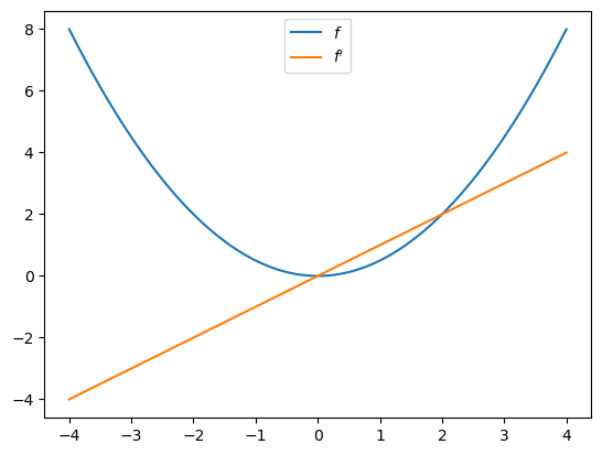
Here’s a very simple illustration, involving the function
def f(x):
    return (x**2) / 2
Let’s take the derivative:
f_prime = jax.grad(f)
f_prime(10.0)
DeviceArray(10., dtype=float64, weak_type=True)
Let’s plot the function and derivative, noting that \(f'(x) = x\).
import matplotlib.pyplot as plt

fig, ax = plt.subplots()
x_grid = jnp.linspace(-4, 4, 200)
ax.plot(x_grid, f(x_grid), label="$f$")
ax.plot(x_grid, [f_prime(x) for x in x_grid], label="$f'$")
ax.legend(loc='upper center')
plt.show()
15.7. Exercises
Exercise 15.1
Recall that Newton’s method for solving for the root of \(f\) involves iterating on
Write a function called newton that takes a function \(f\) plus a guess \(x_0\) and returns an approximate fixed point.
Your newton implementation should use automatic differentiation to calculate \(f'\).
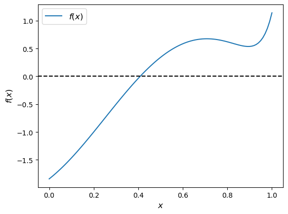
Test your newton method on the function shown below.
f = lambda x: jnp.sin(4 * (x - 1/4)) + x + x**20 - 1
x = jnp.linspace(0, 1, 100)

fig, ax = plt.subplots()
ax.plot(x, f(x), label='$f(x)$')
ax.axhline(ls='--', c='k')
ax.set_xlabel('$x$', fontsize=12)
ax.set_ylabel('$f(x)$', fontsize=12)
ax.legend(fontsize=12)
plt.show()
Solution to Exercise 15.1
Here’s a suitable function:
def newton(f, x_0, tol=1e-5):
    f_prime = jax.grad(f)
    def q(x):
        return x - f(x) / f_prime(x)

    error = tol + 1
    x = x_0
    while error > tol:
        y = q(x)
        error = abs(x - y)
        x = y

    return x
Let’s try it:
newton(f, 0.2)
DeviceArray(0.4082935, dtype=float64, weak_type=True)
This number looks good, given the figure.
Exercise 15.2
In an earlier exercise on parallelization, we used Monte Carlo to price a European call option.
The code was accelerated by Numba-based multithreading.
Try writing a version of this operation for JAX, using all the same parameters.
If you are running your code on a GPU, you should be able to achieve significantly faster exection.
Solution to Exercise 15.2
Here is one solution:
M = 10_000_000

n, β, K = 20, 0.99, 100
μ, ρ, ν, S0, h0 = 0.0001, 0.1, 0.001, 10, 0

@jax.jit
def compute_call_price_jax(β=β,
                           μ=μ,
                           S0=S0,
                           h0=h0,
                           K=K,
                           n=n,
                           ρ=ρ,
                           ν=ν,
                           M=M,
                           key=jax.random.PRNGKey(1)):

    s = jnp.full(M, np.log(S0))
    h = jnp.full(M, h0)
    for t in range(n):
        key, subkey = jax.random.split(key)
        Z = jax.random.normal(subkey, (2, M))
        s = s + μ + jnp.exp(h) * Z[0, :]
        h = ρ * h + ν * Z[1, :]
    expectation = jnp.mean(jnp.maximum(jnp.exp(s) - K, 0))

    return β**n * expectation
Let’s run it once to compile it:
compute_call_price_jax()
DeviceArray(180876.48840921, dtype=float64)
And now let’s time it:
%%time
compute_call_price_jax().block_until_ready()
CPU times: user 2.04 ms, sys: 256 µs, total: 2.3 ms
Wall time: 105 ms
DeviceArray(180876.48840921, dtype=float64)